 |
TORCS
1.3.9
The Open Racing Car Simulator
|


|
|
TORCS
1.3.9
The Open Racing Car Simulator
|
|
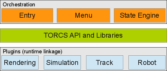
The goal of this chapter is to give an introduction into the major TORCS concepts and components, and to document where you find them in the source tree. The TORCS architecture view presented here identifies 3 major component types. These are components responsible for controlling the major program flow (Orchestration), interfaces and libraries with common code (TORCS API and Libraries) and modules loaded during run time (Plugins).
At start up TORCS goes first through the Entry stage. During this stage the command line is analysed, and depending on the desired operation mode TORCS is run either with a command line specified race configuration file in command line mode (option -r), or the graphical menu is started. The command line mode does not output any graphics, and the simulation time is not synchronized with real time, so this mode is ideal to run simulations without human supervisor as fast as possible. The relevant code is in src/linux/main.cpp for Posix systems, or in src/windows/main.cpp for Windows systems.
The command line mode starts up directly the State Engine in src/libs/raceengineclient/raceinit.cpp, ReRunRaceOnConsole, it is an excellent starting point to review the minimum required setup to start up, run and shutdown the simulation.
The Menu and its components are responsible to offer a visual user interface to ease the setup of TORCS, e.g. the selection of predefined races, changing the selection of robots, graphics and much more. All these settings are persisted in XML files and are read later by the respective components.
The Race menu is a special menu, because the entries presented here are the direct reflection of Race Manager configuration files (look up src/raceman). You can completely customize the Race Manager configuration files if desired (that means adding, removing, renaming and editing), they offer the creation of very simple sessions (e.g. practice.xml) up to full championships (e.g. champ.xml).
When the user finally selects a Race Manager the State Engine is started up in src/libs/raceengineclient/raceinit.cpp, reSelectRaceman.
The State Engine controls the execution of the Race manager specific configuration, setup, run and shutdown of the simulation (src/libs/raceengineclient/racestate.cpp, ReStateManage). To trigger state changes the state of TORCS data can be inspected or for more simple cases the return value of a function call can be considered. Understanding of the State Engine can make some tasks really simple, e.g. implementing a robot which can restart the simulation by itself (not supported by TORCS out of the box, but very easy to add, see TORCS FAQ 6.8).
TORCS defines some interfaces and libraries which are used in multiple parts of the project, e.g. XML parameter file handling, common functions for robots, etc. The header files for the interfaces can be found in src/interfaces, the libraries in src/libs, the most interesting ones for robot programming are parameter handling, robottools, portability, math and learning.
The Plugins share all in common that they have specified interfaces and are loaded based on the configuration during run time, so if you have an alternative plugin you can configure TORCS to use it. As example there are two simulation implementations, simuv2 and simuv3, you can simply change a configuration file to change it. Typical use cases are replacing some of the actual modules with wrappers or adapters, e.g. to run the simulation on MATLAB or to run robots with simulated sensors over the network on other machines (SCR). The interface definitions can be reviewed here.
Rendering (Graphic Module Interface) is responsible for rendering the situation. The current default implementation does visual 3D rendering including sound, based on the OpenGL 1.3 and OpenAL API's. The interface is specified in src/interfaces/graphic.h. The major function is refresh, which takes as argument a struct Situation * and renders it. The code of the actual module is located in src/modules/graphic/ssggraph.
Simulation (Simulation Module Interface) is responsible for progressing the situation by a given time step. The interface is specified in src/interfaces/simu.h. The major function is update, which takes the struct Situation * and simulation timestep (usually RCM_MAX_DT_SIMU) as argument, and progresses the simulation by the time step. The code of the default module is located in src/modules/simu/simuv2.
Track (Track Loader Module Interface) is responsible for loading tracks into the TORCS tTrack structure. The interface is specified in src/interfaces/track.h. The code of the default module is located in src/modules/track.
The robot module(s) (Robot Module Interface) drive the cars in the simulation. TORCS can load multiple robots at the same time to drive multiple cars, one robot supports up to 10 cars at once. The major function is rbDrive, which takes as argument an index of the car to drive with the call, a tCarElt * containing information about the car and a struct Situation * containing the situation. As result the call fills in the tCarCtrl struct, which contains commands to drive the car (steer, brake, accelerator,clutch, ...). The interface is specified in src/interfaces/robot.h. Various drivers implementations are shipped with TORCS, have a look into src/drivers. Specially to mention is the "Human Driver" (human), it takes input from the user to control the car, so if your experiment requires adoption regarding user input have a look at this robot.
The Olethros and bt robot are able to adopt to the track over time and persist the gained knowledge for later runs. If you are interested in other implementations, you can find more robots on The TORCS Racing Board (you can download robots of past events) or on the SCR site.
After discussing the TORCS architecture we are now ready to dig into some details of the simulation loop. This seems to be a topic which is usually not too easy to understand. Let start with taking about time. There are two different times in TORCS, simulation time and real time. The simulation time is basically just the time axis on which we calculate the simulation intermediate results, so if it takes 1 real minute or 1 real ms to simulate 1s in simulation time, the simulation time is just one second, real time does not matter. Real time in contrary is the time observed by the user. So it is very important to understand that the whole TORCS architecture just uses simulation time to perform calculations, evaluation of rules etc., real time does not matter in that respect. Real time is only used to synchronize in some modes simulation time with real time, e.g. to enable a human to drive a car.
The TORCS Simulation Loop starts in the State Engine, src/libs/raceengineclient/racestate.cpp, ReStateManage, case RE_STATE_RACE. In mode=ReUpdate(); everything is performed, and if the race is still normally running the State Engine while loop will return into the same state again and again, till some condition for a state change is fulfilled (e.g. when the race has ended).
ReUpdate is located in src/libs/raceengineclient/raceengine.cpp. It has four distinct operating modes:
RM_DISP_MODE_NORMAL: This mode is mostly suitable for interactive simulations, it takes into account simulation time and real time. It basically works like this: Progress the simulation time until simulation time has caught up with real time, then render a frame.
Now this has some consequences, because TORCS is usually not the only running process in the operating environment and is usually not running as real time task. So if another process or the operating environment hooks up some resources, it might happen that TORCS sleeps for a moment, and after that nap it has to catch up. So a consequence of this mode is that even if you repeat runs of the exact same simulation in simulation time, that the rendered frames will quite likely not be the identical ones. This can have as well an impact on human player performance, if some frames take very long to appear.
If you want to simulate a video source with exactly one frame every X seconds RM_DISP_MODE_CAPTURE might be a better solution. RM_DISP_MODE_NORMAL mode has two more features: If the simulation lags behind a lot and is not able to catch up, it spits out at least a frame on every 2000th time step, this is required to keep the GUI interactive (processing the event queue). There is as well a time warp (up to 128 times real time) and slow motion mode (down to 1/64 times real time).
RM_DISP_MODE_NONE: This mode is used for the "blind mode" in practice sessions, it does just consider simulation time, no 3D scenery is rendered. Every 2 seconds of simulation time the list in the GUI regarding the current progress is updated. This mode is suitable for development of robots. You can run experiments with almost no overhead, but you can switch quickly in the GUI between runs from and back to RM_DISP_MODE_NORMAL to investigate problems.
RM_DISP_MODE_CAPTURE: This mode is used to capture frames at exact points in simulation time (e.g. every 0.03s). The time is not synchronized with real time, so the simulation might be faster or slower than real time, depending on the load you generate. Time warp and slow motion modes are available as well. This would be with some little modification the most suitable mode for creating an AI driving based on video frames.
RM_DISP_MODE_CONSOLE: This mode is used when you start TORCS with the -r option from the command line, it does have no GUI at all, it just prints out some progress information. This mode is intended for batch operation and unit testing.
As you can see in all these modes, ReOneStep in src/libs/raceengineclient/raceengine.cpp is then called at some point, this actually executes the simulation time step. Here is a good point to set a break point to investigate the call stack when you are new to the TORCS code base.
The discretisation and simulation loop has another consequence which is to consider: Lets assume that we disable everything which changes car properties, so we have no damage, use no fuel, etc. Now you would expect that a non learning, perfect controlled, hard coded robot would drive lap by lap the same lap (and lap time), would you? But that is not the case. Lets assume that we hit on our Nth lap accidently exactly the starting line with the car center, and let us draw a point on every simulated time step on the track. Now when we finish the Nth lap it is very unlikely that we hit exactly the same point where we started because of time discretisation, so every consecutive lap will be similar but not identical.
Simulation time limits: Because the simulation time is represented as double, and the simulation time step is finite (RCM_MAX_DT_SIMU) applications are expected to run stable up to 1 Million Days simulation time (the simulation core itself does only depend on the time step, so it would run stable for ever). The longest known performed experiments are 100000 km races in command line mode.
 1.8.14